Mapping Flood Impact in Nepal with Sentinel-2

Overview

In late August 2026, intense monsoon rainfall triggered flooding and debris flows along river corridors in central Nepal. In this project I explore how freely available Sentinel-2 imagery and QGIS can be used to map the visible impact of the event, and to check which infrastructure lies within the mapped flood-affected area.

In short: about 11.5 km² of the study area shows surface change linked to the late-August event, as mapped on 21 September 2026. About 3,900 buildings, 98 km of roads and tracks, 62 points of interest and 88 bridge segments touch this mapped area (potential exposure, not confirmed damage).

I compared satellite images from before and after the event, combined spectral indices with visual interpretation, and then overlaid roads, buildings and facilities. One challenge shaped the whole project: the first clear post-event image was taken about 25 days after the event (flooding was observed on 27 August), when much of the water had already drained away.

Disclaimer: This is a desktop study based on Sentinel-2 satellite imagery at 10 m resolution, so the results are indicative and may not be exact. Ground-based or survey-level data could show different extents, damage and impacts. Please do not use these maps for emergency response, insurance or planning decisions.

Study area and data

The study area is a ~90 km² corridor along the Trishuli River, from the upper Trishuli (Bhote Koshi) in Rasuwa downstream to its confluences with the Budhi Gandaki and Marsyangdi. The boundary is the HOT flood-corridor polygon, so the percentages below are shares of that corridor, not of the whole river basin.

Two Sentinel-2 Level-2A images were used:

• Before: 12 August 2026
• After: 21 September 2026

The imagery came from the Copernicus Browser, and all processing and mapping was done in QGIS. Roads, facilities and rivers came from OpenStreetMap; building footprints from OpenStreetMap, Google Open Buildings and Microsoft. The Copernicus GLO-30 DSM (a surface model, so it includes trees and buildings) was used as a terrain check: height above the nearest mapped river, and slope. The 27 August flooding date comes from a HOT/OpenStreetMap flood-extent polygon, which was used for context only. Copernicus Emergency Management Service activation EMSR927 and two Sentinel-1 radar scenes (16 and 28 August) were used afterwards to cross-check the result, not to build it.

1. Preparing the imagery

The study area covers four Sentinel-2 tiles. For each date I joined (mosaicked) the tiles separately for the five bands I needed: blue (B02), green (B03), red (B04), near-infrared (B08) and short-wave infrared (B11). From these I built true-colour and false-colour images for both dates. B02, B03, B04 and B08 are delivered at 10 m, but B11 is delivered at 20 m, so I resampled it to 10 m (bilinear). That makes the pixels line up, but it does not add detail: the water index below is effectively a 20 m measurement shown on a 10 m grid.

2. Reading the landscape first

Before running any analysis, I simply looked. Drag the slider to compare the same place before and after the flood:

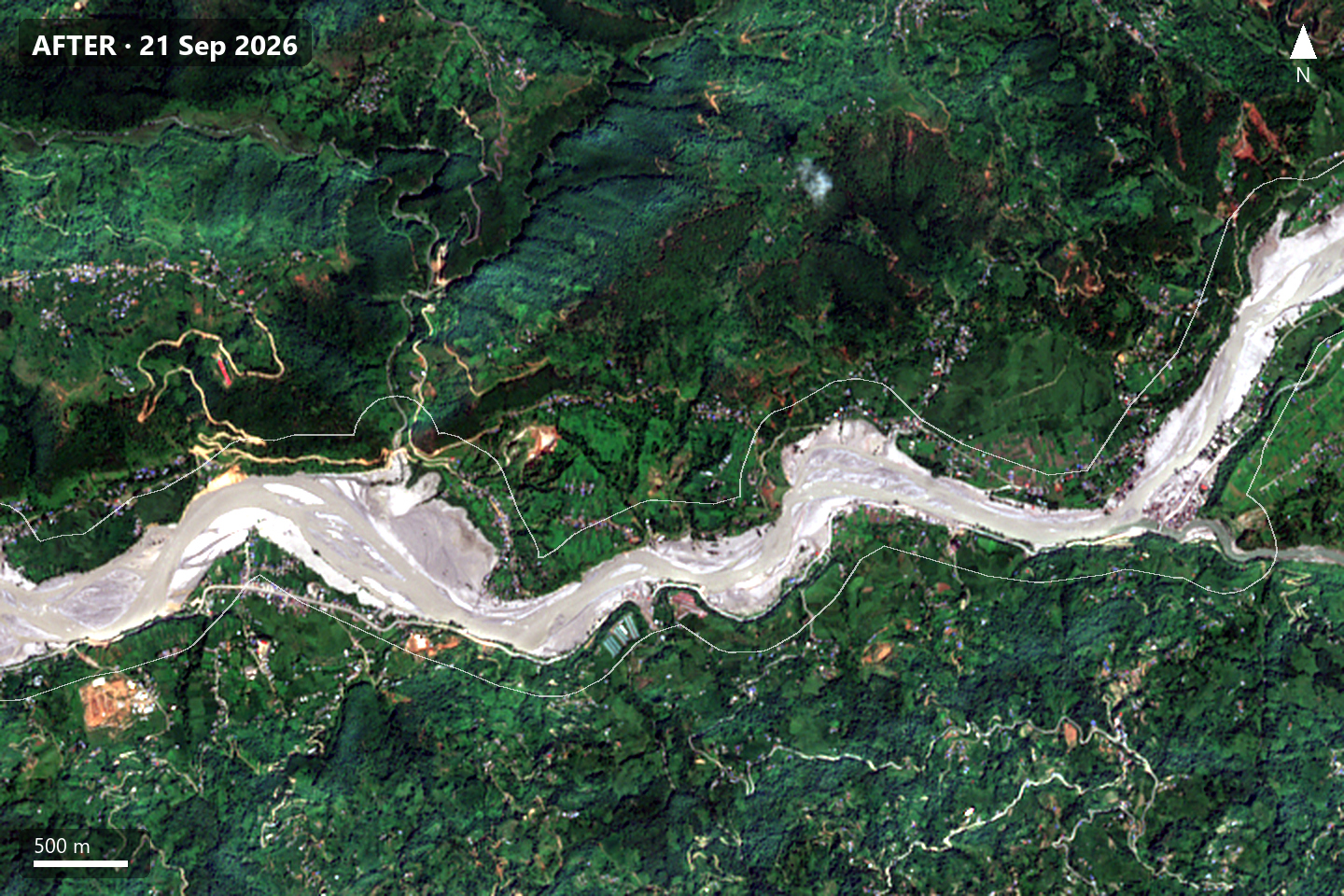
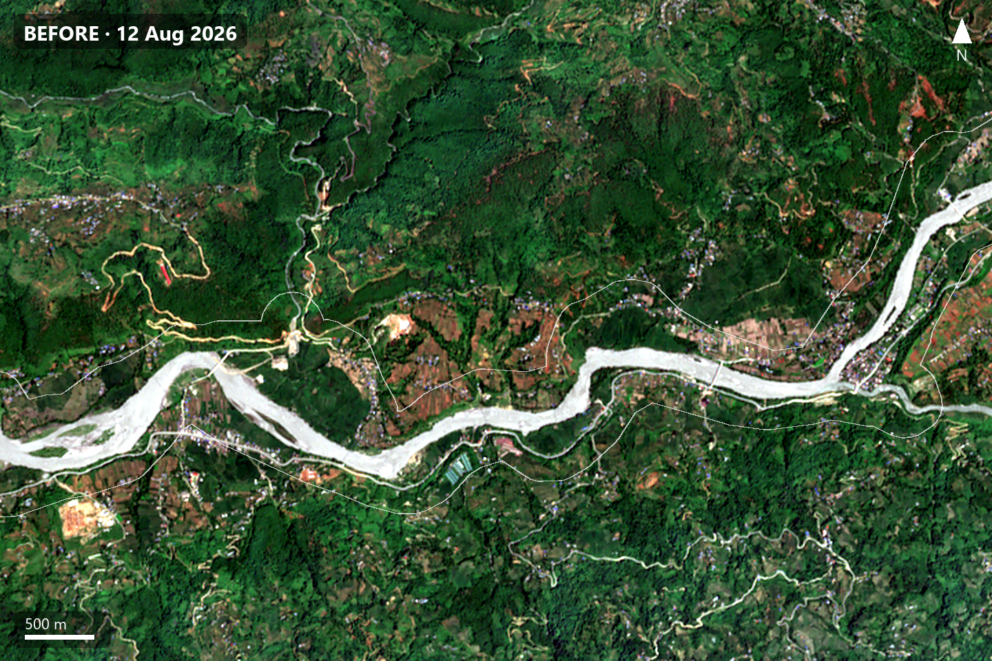
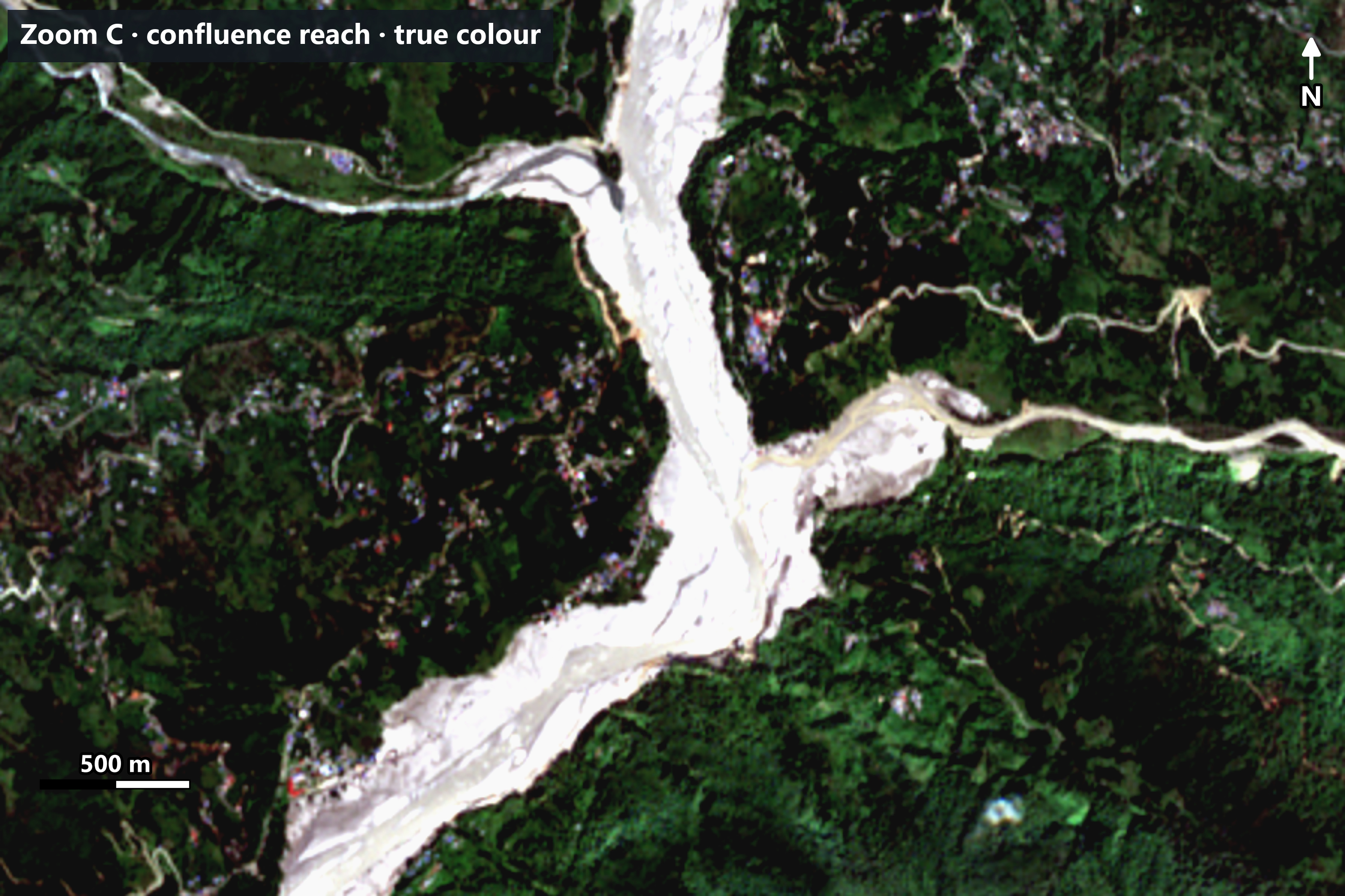
The river channel is much wider, and fields and trees next to it have been replaced by pale grey-brown surfaces, consistent with sediment and debris left by the flood.

A false-colour image helps even more. It shows near-infrared light as red, and healthy plants reflect a lot of near-infrared, so vegetation glows red while water and fresh sediment appear cyan:

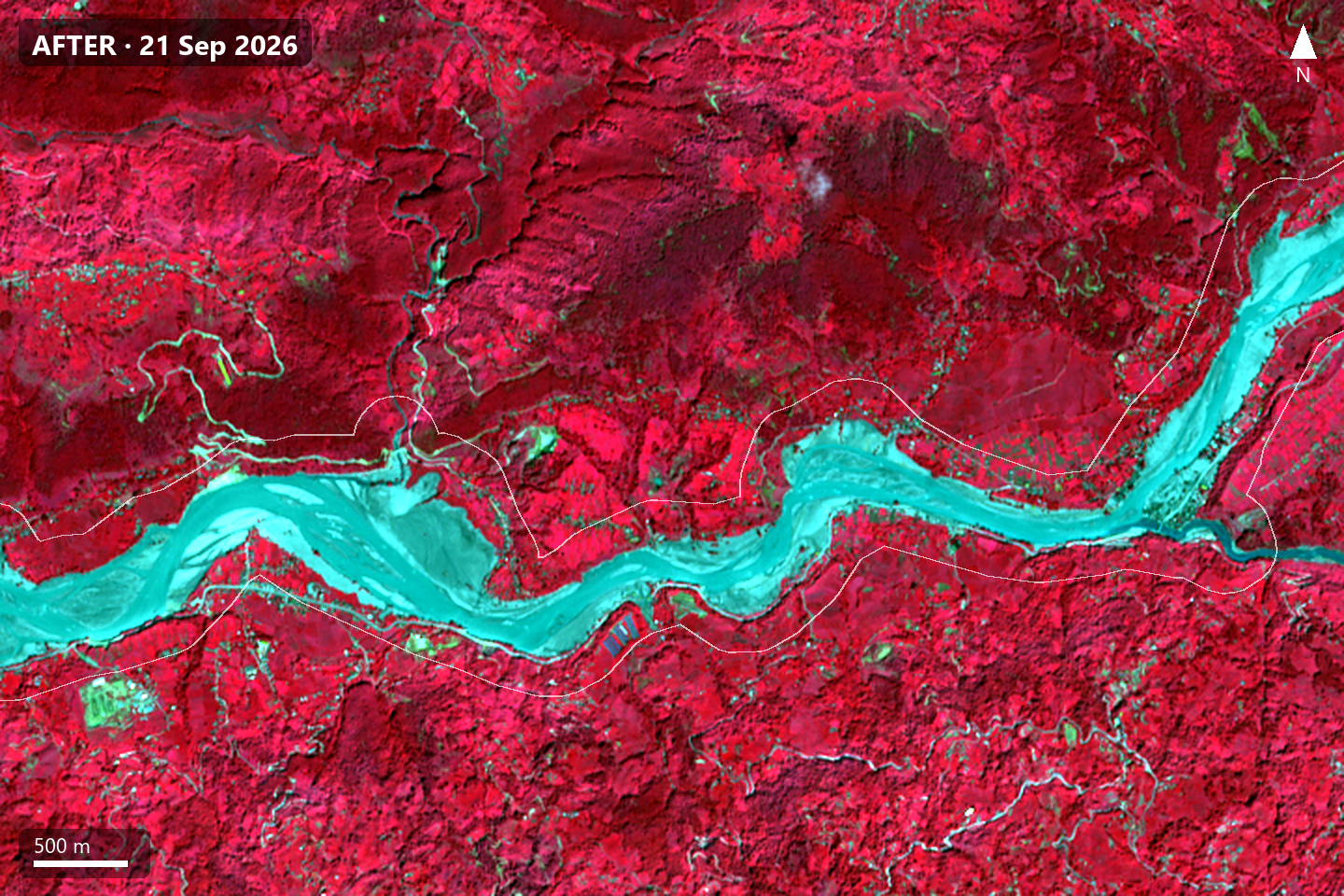
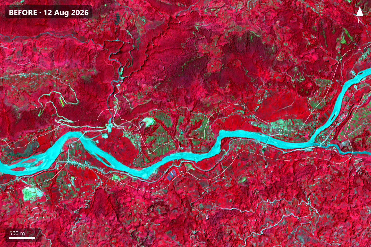
3. Mapping water with MNDWI

To let the computer find water, I used the Modified Normalized Difference Water Index (MNDWI):

MNDWI = (Green − SWIR) / (Green + SWIR)

Water absorbs short-wave infrared, so water pixels have MNDWI above 0. I used a threshold of 0 for both dates, then looked for pixels that were water after the event but not before.

The threshold matters. Moving it by ±0.1 changes the raw new-water area between about 2.9 and 4.4 km² (3.3 km² at 0). Water also disappeared from about 2.4 km² (river shifts and falling levels), so the net change in mapped water is only about +0.9 km².

Note: Indicative result from 10 m Sentinel-2 imagery. It may not match field or survey-level data.

4. Why the water map was smaller than the visible damage

The MNDWI result was much smaller than the area that looked affected in the photos. At first I thought I had made a mistake.

The acquisition date explained it. By 21 September much of the floodwater had drained, and areas that had been flooded were now mud, sand, silt and gravel rather than water. The pixel values confirmed it: the grey-brown surfaces reflected about four times more short-wave infrared than a typical water pixel (the median of all pixels mapped as water). Because MNDWI relies on water absorbing SWIR, these surfaces could never appear as water.

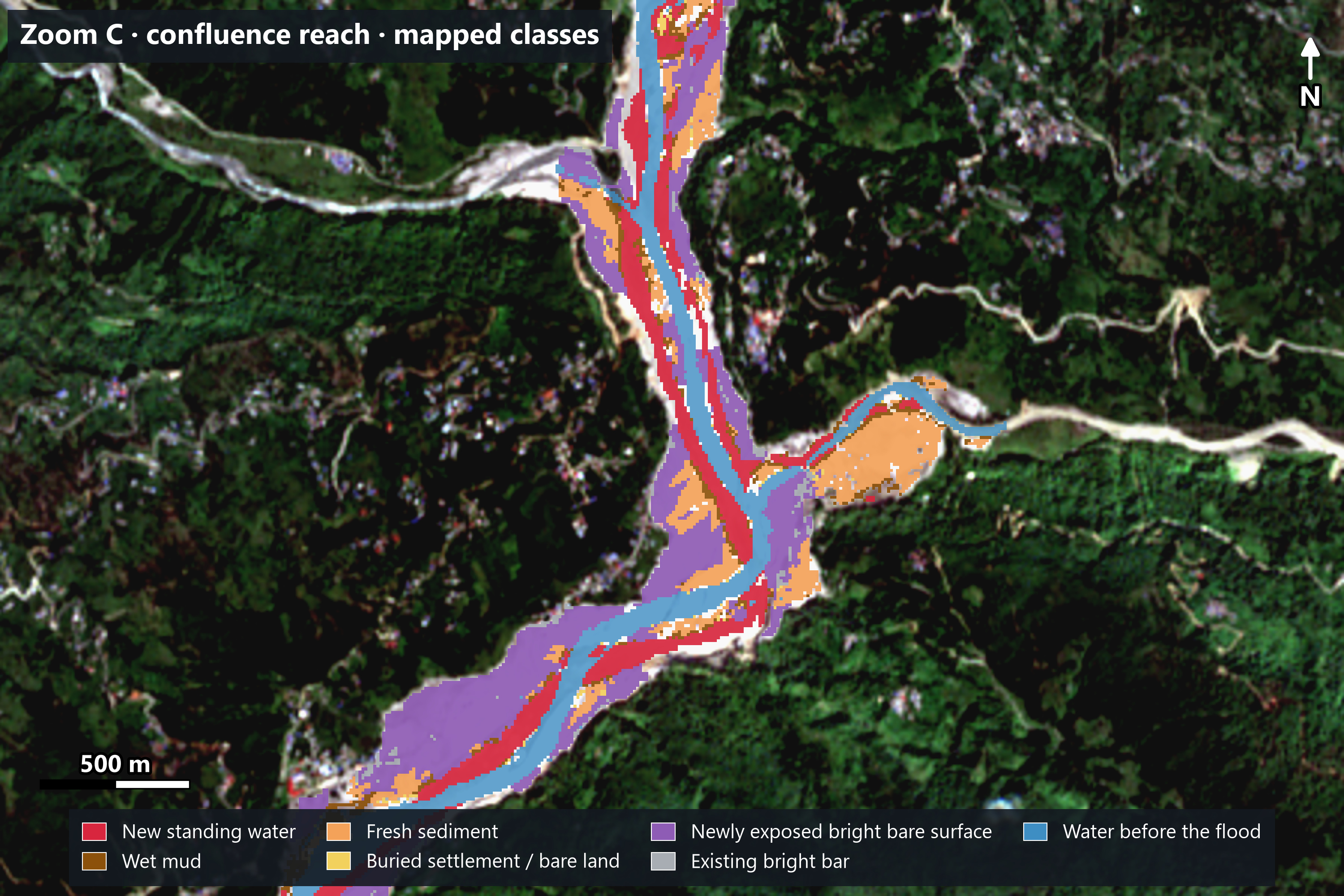
So instead of treating the water map as the whole flood footprint, I split the result into three parts: new standing water, land showing signs of flood sediment, and newly exposed bright bare surface.

5. Mapping flood-affected sediment

I added a second rule to catch areas that were clearly affected but no longer underwater. It mainly looks for places that were vegetated before and bare grey-brown after, on low ground next to the river. A smaller extra rule catches settlements, bare plots and small ponds buried by fresh sediment (about 0.24 km²).

A third land class covers newly exposed bright bare surface: bright, bare, non-water ground near the river or the other flood classes that changed clearly between 12 August and 21 September (about 0.18 reflectance after the flood against 0.07 before, as class averages). Most of it was vegetated before, and much of it lies on banks, terraces and slopes, so it can include debris-flow and landslide deposits as well as sand and gravel. I count it in the total but treat it as lower confidence. Surfaces that were already bright before the flood (little change) are drawn in grey as existing bright bar and are not counted.

These thresholds came from the spectral behaviour and terrain I observed. They were not fitted to a training dataset, so they are rules for this case study, not universal values.

6. Cleaning up false alarms

The first results contained mistakes, so I filtered them:

• removed clouds and cloud shadows
• removed steep hillsides high above the river from the water and sediment classes, where mountain shadows and landslide scars can mimic flood effects (the bright bare surface class has no terrain limit)
• removed tiny patches smaller than about 0.1 hectare (applied to the merged water and sediment classes, and to the bare-surface class before it was smoothed)
• excluded water that was already there before the flood
• checked the results against the before and after images

7. The result

Note: Indicative result from 10 m Sentinel-2 imagery. It may not match field or survey-level data.

Drag the slider to compare the true-colour image (left) with the same view and the mapped classes (right). Red = new standing water, brown = wet mud, orange = fresh sediment, purple = newly exposed bright bare surface, grey = existing bright bar, blue = water before the flood.

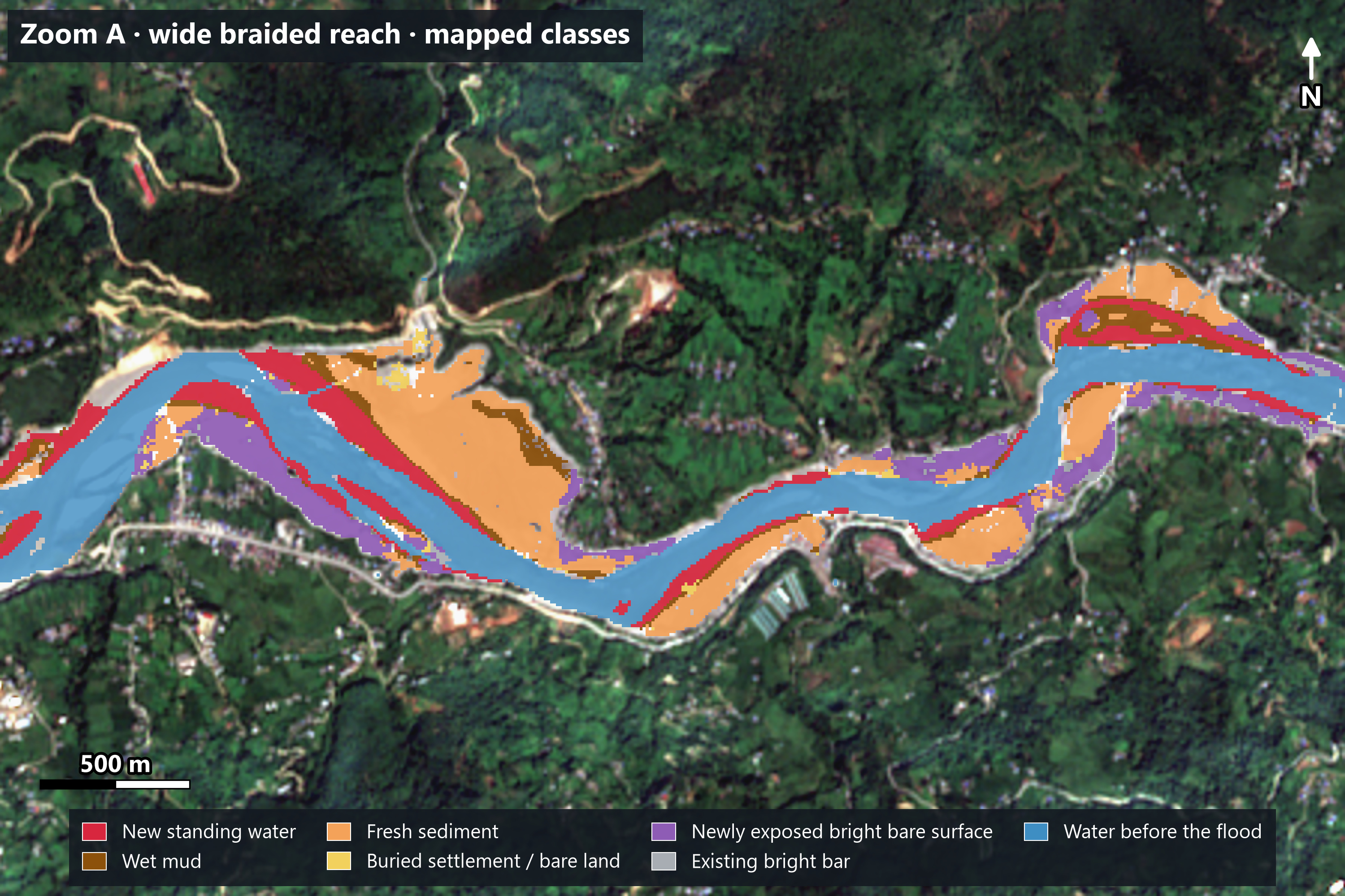
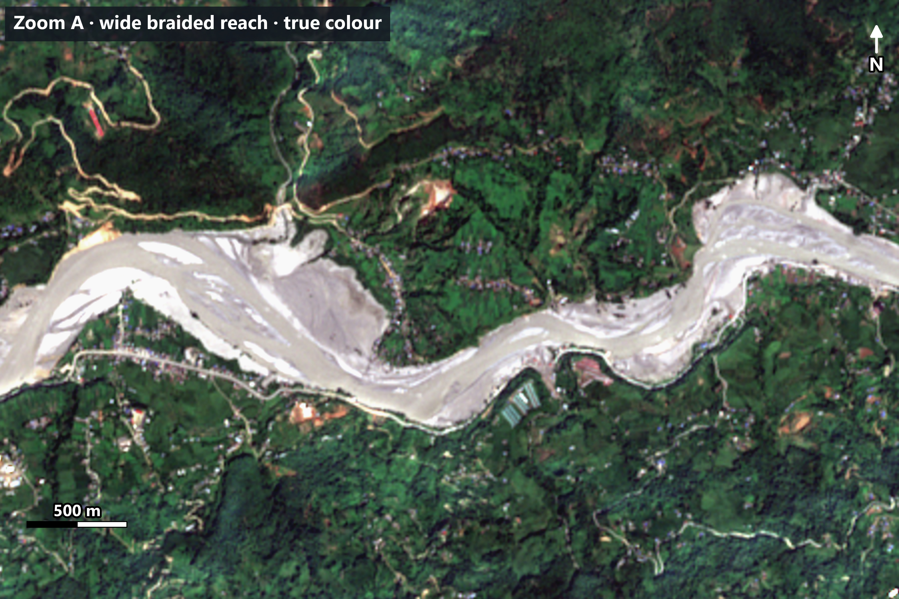
Note: Indicative result from 10 m Sentinel-2 imagery. It may not match field or survey-level data.

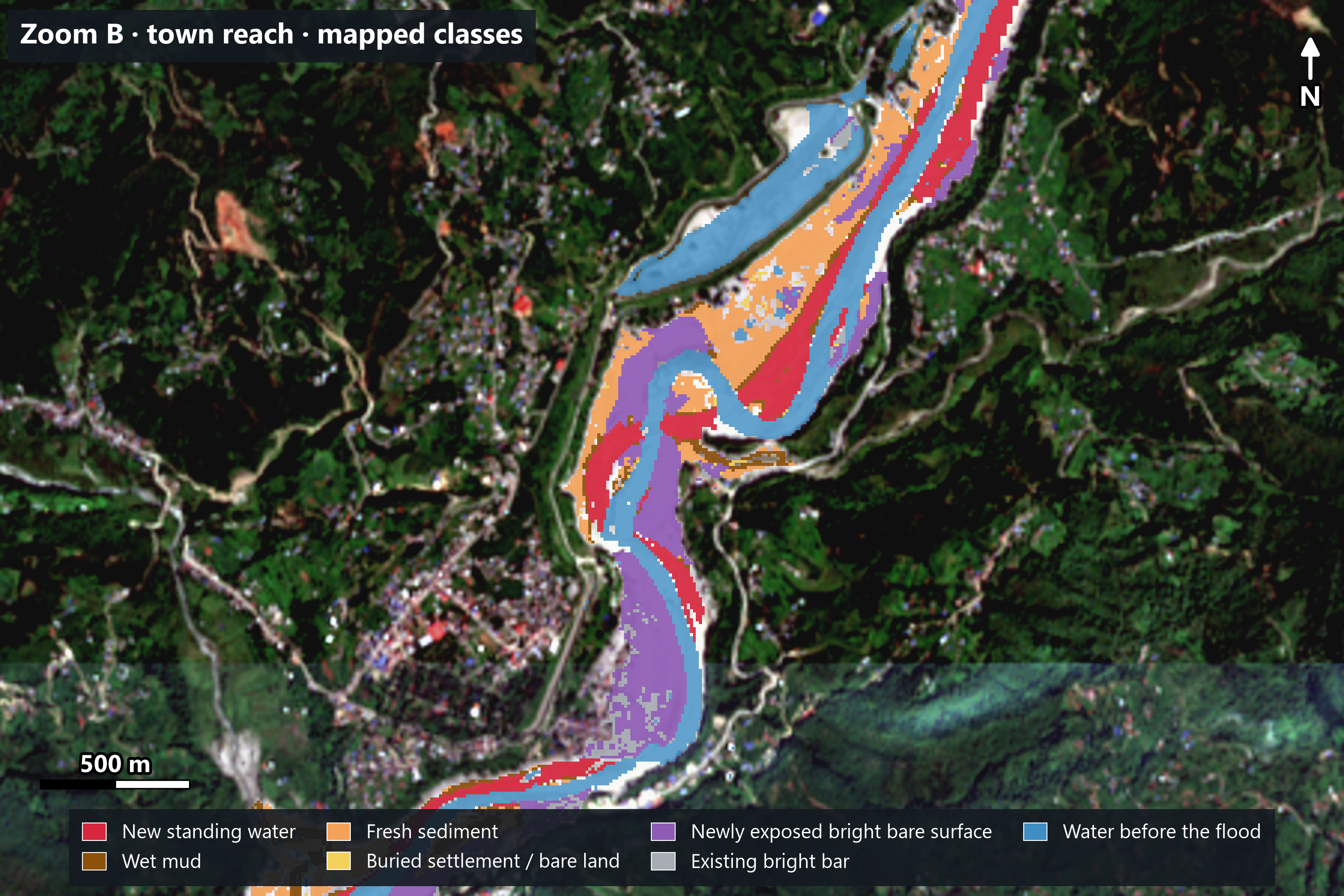
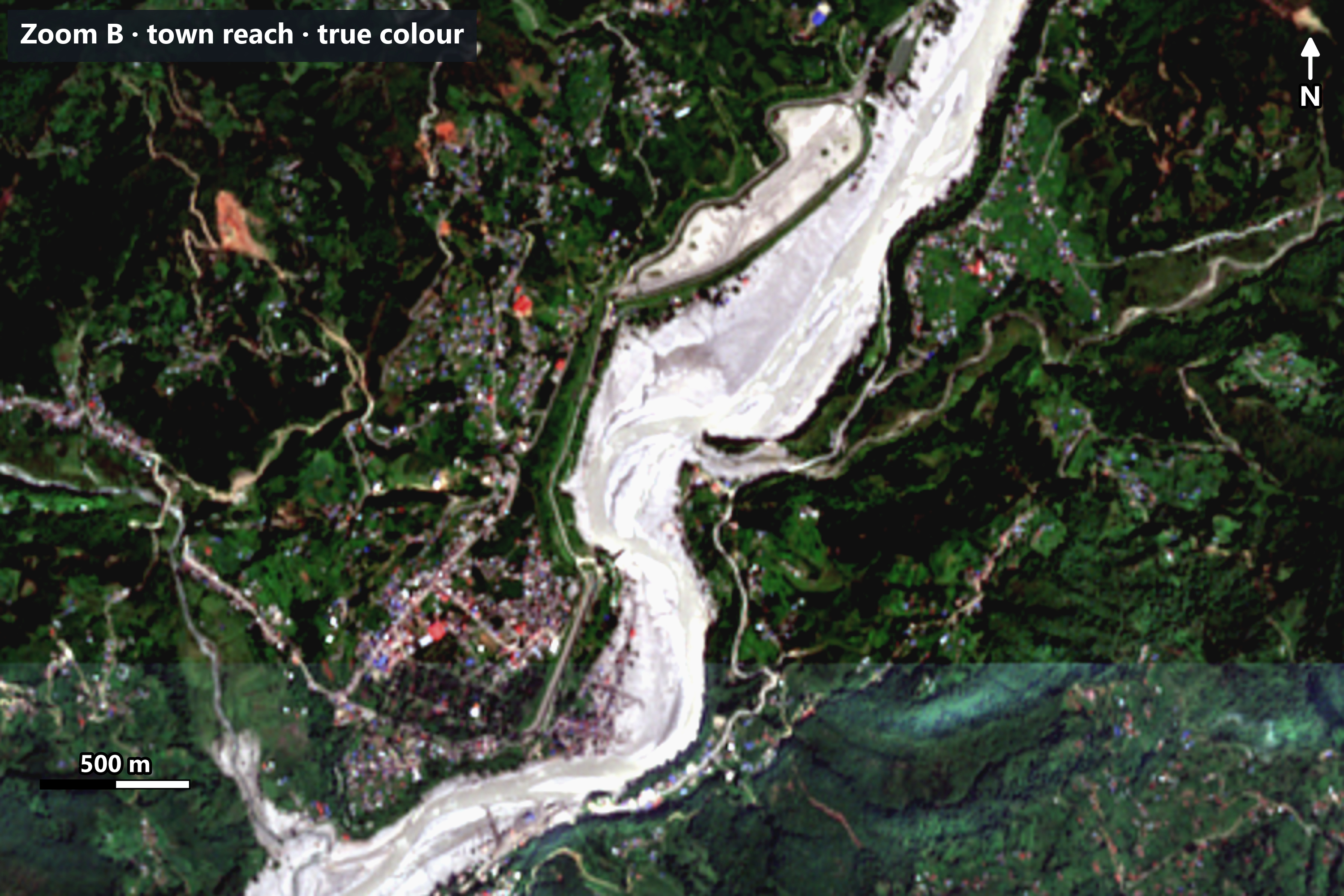
Note: Indicative result from 10 m Sentinel-2 imagery. It may not match field or survey-level data.

Note: Indicative result from 10 m Sentinel-2 imagery. It may not match field or survey-level data.

Mapped class	Area
New standing water (indicative)	2.1 km²
Sediment and mud on land (indicative)	3.2 km²
Newly exposed bright bare surface (lower confidence)	6.1 km²
Total mapped surface change	11.5 km² (about 13% of the study area)

Class areas are rounded; unrounded they are 2.144 + 3.178 + 6.135 = 11.457 km². Cloud, shadow and no-data pixels (7.9 km², 8.7% of the corridor) could not be assessed, so the share is 12.7% of the corridor, or 13.9% of the area that could be assessed.

At 10 m resolution, standing water and wet mud are often hard to tell apart, so the split between those two classes is indicative. The total is the main result, and it is fairly stable: reasonable changes to the terrain, cloud-buffer and patch-size settings move it by about ±2%, while the water threshold moves it by about −8% to +6%. The split between the sediment and bare-surface classes depends much more on the settings. Another 1.0 km² of bright bars that were already there before the flood is shown in grey and not counted.

The image was taken about 25 days after the flood, so 11.5 km² shows what remained visible then, not the peak flood extent.

Two other records help with timing. Sentinel-1 radar backscatter in the water and sediment classes had already changed by 28 August, one day after the reported flood, compared with almost no change in vegetated land. And 27 August is the date of the first very-high-resolution images (the HOT polygon and Copernicus EMS imagery), so the event itself may have started earlier.

8. What's inside the flooded area?

I overlaid infrastructure data on the mapped surface-change area:

Infrastructure	Potentially exposed
Buildings	3,886 of 18,200 (any part touches the mapped area)
Roads and tracks (OSM, including footpaths)	97.7 km of 562 km
Points of interest (OSM amenities, shops, tourism, man-made)	62 of 401
Bridge segments (OSM lines)	88 of 147

Note: Indicative result from 10 m Sentinel-2 imagery. It may not match field or survey-level data.

These features touch the mapped surface-change area: they are potentially exposed to mapped flood-related change. About 63% of the exposed buildings (2,438 of 3,886) and 60% of the exposed road length (59 of 98 km) touch the lower-confidence bare-surface class. The counts depend on the rule used: counting only buildings whose centre falls inside the mapped area gives about 3,200, and counting only the water and sediment classes gives about 1,600. For bridges, 88 of 147 lines touch the area, but only 26 have their midpoint inside it. Only 25 of the 401 points of interest are utility-type features; most are schools, hotels, restaurants and shops.

As a cross-check, Copernicus EMS (EMSR927) graded buildings and roads from 0.3 to 1 m imagery in parts of the corridor. Roads it graded "no visible damage" almost never touch the mapped area (0.1% of their length), while 56% of the length it graded "destroyed" does, and about 89% of buildings it graded "destroyed" lie within 20 m of it. That shows the map follows real impact, but satellite imagery at 10 m cannot show whether an individual building or road was damaged or washed away, so these are counts of exposure, not confirmed damage.

Key takeaways

• Timing matters. An image taken 25 days after a flood shows what the flood left behind, not the flood itself.
• Look before you calculate. True and false colour images revealed changes the water index missed.
• MNDWI finds water, not flood impact. Once the water has drained, it can't show the full footprint.
• Combine evidence. Spectral change plus terrain and context gives a fuller picture.
• Filters are a trade-off. The rule that removed false alarms also removed some real flood areas.

Limitations

• The 21 September image shows conditions about 25 days after the event, not the maximum flood extent.
• Clouds and shadows can hide or distort the ground.
• The MNDWI > 0 threshold suits these images but may need adjusting elsewhere.
• The sediment and bare-surface rules are case-specific, not a universal classifier.
• The newly exposed bright bare surface class (6.1 km²) is defined only by brightness, change between two dates and distance to the river or the other flood classes. It is not a sand or gravel classification, and it can include landslide and debris-flow scars.
• Flood, debris flow and landslide effects cannot be separated with two images; Copernicus EMS maps this event as landslides.
• Sun angle and season differ between the two dates (more terrain shadow in September).
• Band B11 is 20 m resampled to 10 m, and the elevation data is a surface model, not a bare-earth model.
• Filtering removes false alarms but also some genuine flood areas.
• Standing water and wet mud look alike at 10 m, so the class split is indicative.
• Features inside the mapped area were exposed to the flood; the actual damage cannot be confirmed from 10 m imagery.
• The map has not been checked against field or survey data. A visual check of 178 points against the same Sentinel-2 images, and the EMS comparison above, show it follows the mapped event, but neither is an independent accuracy assessment.
• 10 m pixels can't show very small features or narrow channels.
• The 12 August "before" image is itself in the monsoon, so some water may already have been above normal.

Data and tools

• Imagery: Sentinel-2 Level-2A, Copernicus / European Space Agency
• Elevation: Copernicus GLO-30 DSM
• Study-area boundary: HOT flood corridor
• Roads, points of interest, bridges, rivers: © OpenStreetMap contributors (via HOT exports)
• Buildings: OpenStreetMap contributors, Google Open Buildings, Microsoft ML Buildings (merged HOT export)
• Flood extent observed 27 August: HOT/OpenStreetMap (context only)
• Cross-checks: Copernicus Emergency Management Service activation EMSR927; Sentinel-1 radar data, Copernicus / ESA
• Boundaries: Nepal standard administrative shapefiles
• Software: QGIS

---