

Land Conversion Around Bengaluru: Mapping Built-Up Growth with Sentinel-2, 2018 to 2026
How much land around Bengaluru became built-up between 2018 and 2026, where it happened, what a 10 m satellite map can and cannot show, and how I checked it against my own labels
Introduction
Bengaluru keeps growing into the farmland around it. I wanted to measure how fast that happened between 2018 and 2026 in the Bengaluru Metropolitan Region, which covers Bengaluru Urban, Bengaluru Rural and Ramanagara districts, using free Sentinel-2 imagery. I also wanted to know how far the answer can be trusted.
In short: the satellite map shows built-up land growing from about 630 km² in 2018 to about 1,080 km² in 2026. That map is too high. When I checked it against points that I labelled by eye on high-resolution imagery (300 in a first round and 150 on a fresh sample), the area that was really built up in 2026 came out at about 720 km² (plus or minus 110 km²). The land built up in 2018 was about 530 km² (plus or minus 120 km²). That puts new built-up land at roughly 190 km² (plus or minus 75 km²), about a third more than in 2018. If cleared plots without buildings count, the figure is about 260 km², roughly 70 km² more.
On the map, most of the new land is 10 to 30 km from the city centre, and a third of it sits within 500 m of a major road.
Disclaimer: This is a desktop study using Sentinel-2 imagery at 10 m resolution and reference land-cover maps. It measures land cover, not legal land use, and it is not a land-records study. The results are indicative. Please do not use them for property, legal or planning decisions.
What is land conversion, and what can a satellite see of it?
"Land conversion" usually means farmland or open land that becomes something else, most often housing, roads and industry. A government record of conversion is a legal change of land use. A satellite sees something different: it sees that a patch of ground looked like a field in one year and like roofs or paved ground in another.
A plot can be cleared, levelled and sold without a single building on it. The satellite may show bare soil, and the land record may show conversion. In this study I count land as converted only when the surface looks built, and I report cleared plots separately.
The imagery comes from Sentinel-2, a set of European satellites that image most of the world's land every few days at 10 m resolution in the visible and near-infrared bands. Each pixel is a 10 m by 10 m square. A typical Indian house is only a few pixels wide, so many pixels are a mixture of roof, road, tree and soil. That mixing turned out to be the main limit of the study.
Why Bengaluru
The region is large (about 7,900 km² in the boundary data I used; the official figure is 8,005 km²) and its edge is changing. Farmland, rocky hills, lakes and plantations sit next to dense neighbourhoods and new layouts. That mix is a hard test for a land-cover map.
I used three time points, 2018, 2022 and 2026, and not every year. A year-by-year series looks richer, but each year brings its own cloud, haze and dryness, and the differences between years can look like change. Three points four years apart keep the picture simple.
Legend
How the map is made
Composites
For each year I took every clear Sentinel-2 observation from January to March and combined them with a median. That is the dry season, which has the fewest clouds. A median ignores the odd cloudy or hazy value.
A problem with the older archive
Newer Sentinel-2 scenes store brightness with a +1,000 offset, and the metadata tells you to subtract 0.1 from the reflectance. In the older archive I used for 2018 and 2022, many scenes carry that instruction in their metadata but their values do not contain the offset. Following the metadata made those scenes about 0.1 too dark. I tested lake pixels instead, which should be nearly black in the short-wave infrared, and applied the correction only to scenes whose lakes showed the offset.
Why not NDBI
The textbook index for built-up land is NDBI, which compares the short-wave infrared band to the near-infrared band. It does not work well here. In the dry season, bare fields and dry grass reflect strongly in the short-wave infrared, so they score as high as, or higher than, the buildings. In my test the index separated built-up land from farmland worse than chance.
The classifier
Instead I trained a machine-learning classifier, a model that learns from examples which combinations of band values look built. I trained it on places where two reference maps, ESRI 10 m land cover and ESA WorldCover, agree. I kept only pixels whose eight neighbours had the same label, so the examples were pure.
Calibrating each year
The same classifier gives different false-positive rates in different years, because the composites differ. I set each year's cut-off so that land that is certainly not built (farmland far from any buildings) gets the same false-positive rate in every year. A pixel then counts as built in a year only if it is also built at the next date, and once built it stays built.
What the map shows
Built-up land (mapped)
Note: Mapped areas over-count built-up land. Use the map for where growth happens, and the accuracy section for how much.
The core is already dense in 2018. New land appears around it, along the roads and next to the smaller towns.
How far from the centre
On the map, the 15 to 20 km ring went from about 13% built in 2018 to about 30% in 2026, and the 20 to 25 km ring from 7% to 16%. Most of the new land sits in the rings from 10 to 30 km. Beyond 40 km the built share rose by only a few points.
Along the roads
I downloaded the motorways, trunk roads and primary roads from OpenStreetMap and measured the distance from each mapped new-built cell to the nearest one. About a third of the new land (34%) lies within 500 m of a major road, on land that makes up only 18% of the region. About half (52%) lies within 1 km of one.
The corridor with the most new land within 2 km is NH 44, the Bellary Road toward the airport, with about 11% of all new land on the map. NH 648, SH 35, NH 48 and SH 104 follow. Growth relative to the land available is highest along SH 104, SH 35 and NH 44.
Which taluks
Bengaluru South adds the most land (+98 km² on the map), followed by Anekal (+62 km²) and Bengaluru North (+59 km²). The two Bengaluru taluks are the largest and already the most built, so their percentages are small. In percentage terms the fastest growth is at the edge: Devanahalli (about 14 to 40 km² on the map, +193%), Yelahanka (+182%) and Hoskote (+155%). Anekal roughly doubles, from 52 to 114 km².
What the new land was before
What was the new built-up land before? The two reference maps disagree. ESRI's 2018 map, the start of the period, shows 63% of it as already built (280 km² of the roughly 445 km² mapped), 25% as cropland (110 km²) and 11% as other vegetation. WorldCover 2020 shows 31% as cropland (137 km²), 32% as already built, 19% as bare ground and 18% as other vegetation. So I cannot say that most of the new land was farmland. (An earlier version of this post read ESRI's 2021 and 2023 maps, which fall inside the period, and so showed 81% as already built.) The part that was farmland is small next to the farmland that exists: ESRI's 2018 map has about 3,620 km² of cropland in the region, of which about 110 km² (3.0%) is now mapped built. WorldCover's 2020 map has about 2,990 km², of which about 137 km² (4.6%) is now mapped built. Conversion is highest 10 to 20 km from the centre, where 12% to 26% of the farmland on the two maps became built-up land, and falls to about 2% or less beyond 40 km.
Because the map over-counts new built-up land, these farmland numbers are upper bounds. In the validation sample, the map's new-built area was about 2.3 times what my labels support.
Three places
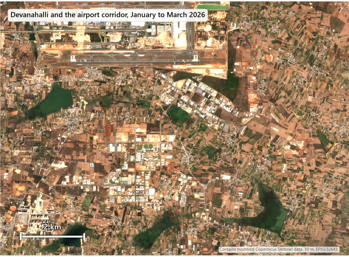
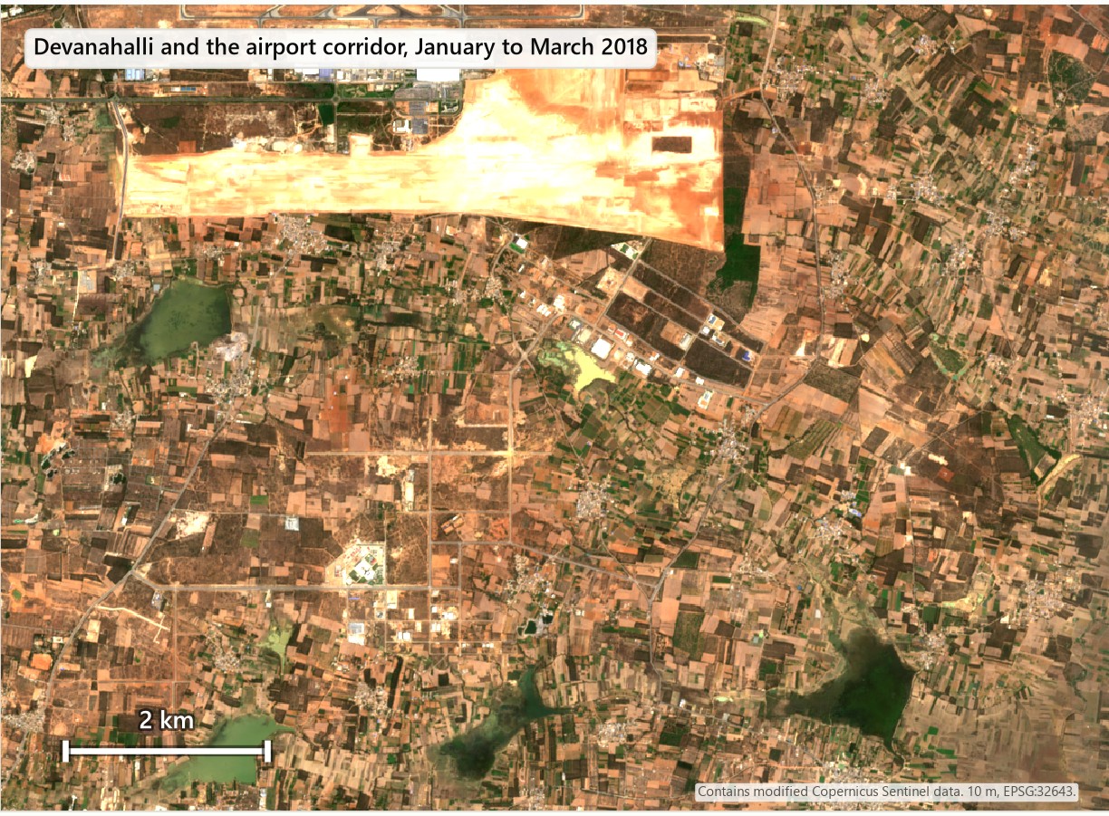
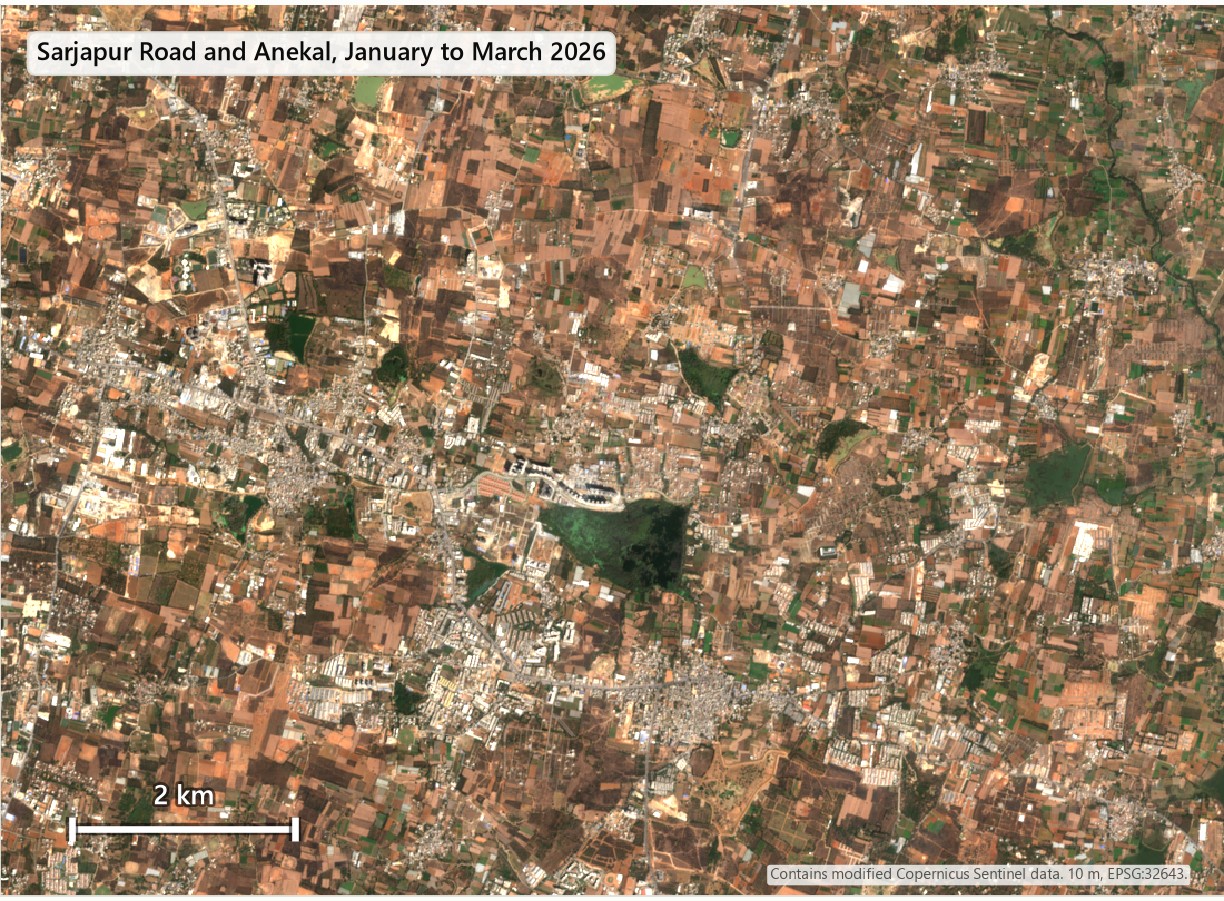
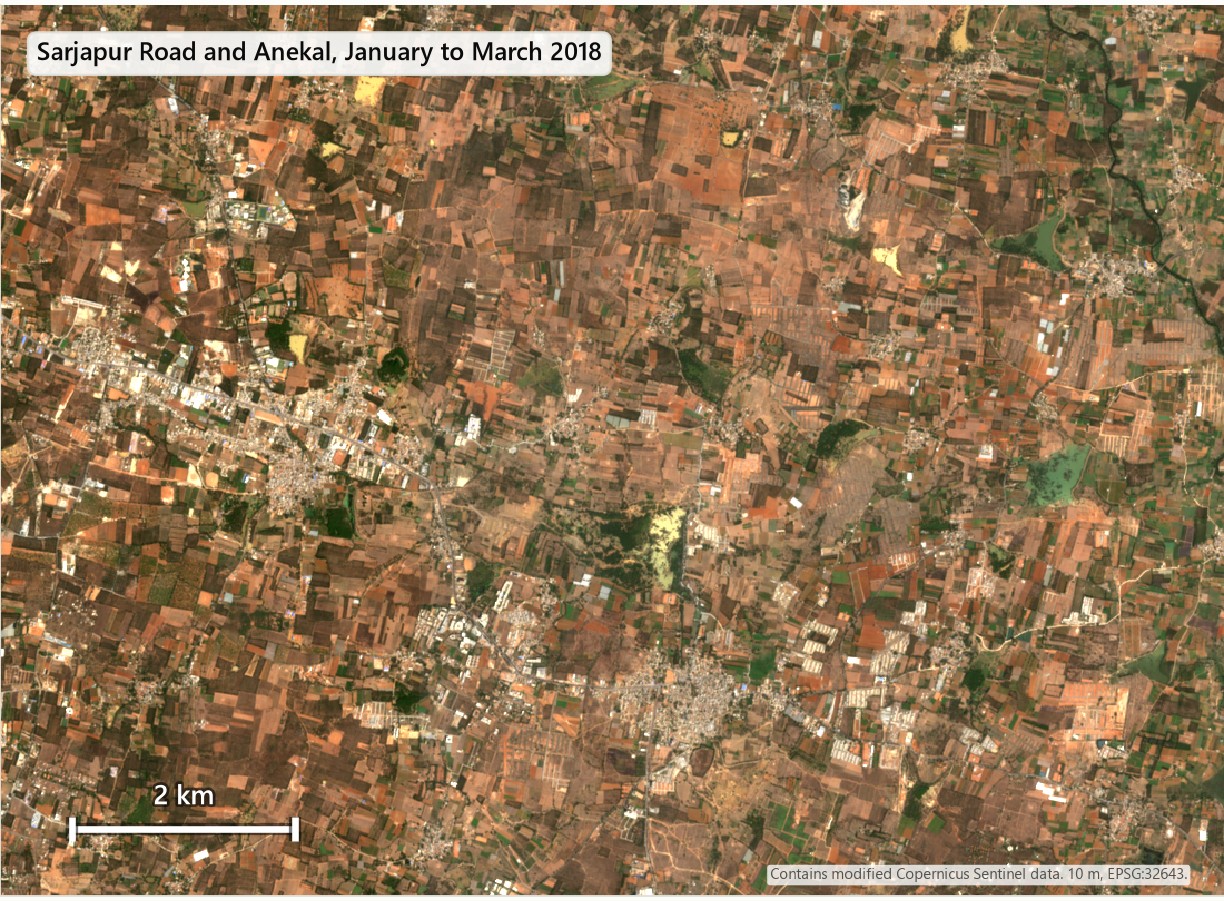
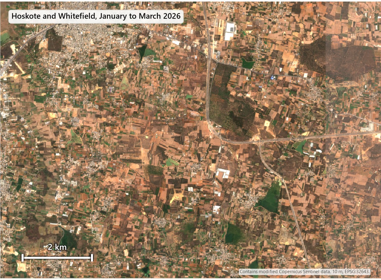
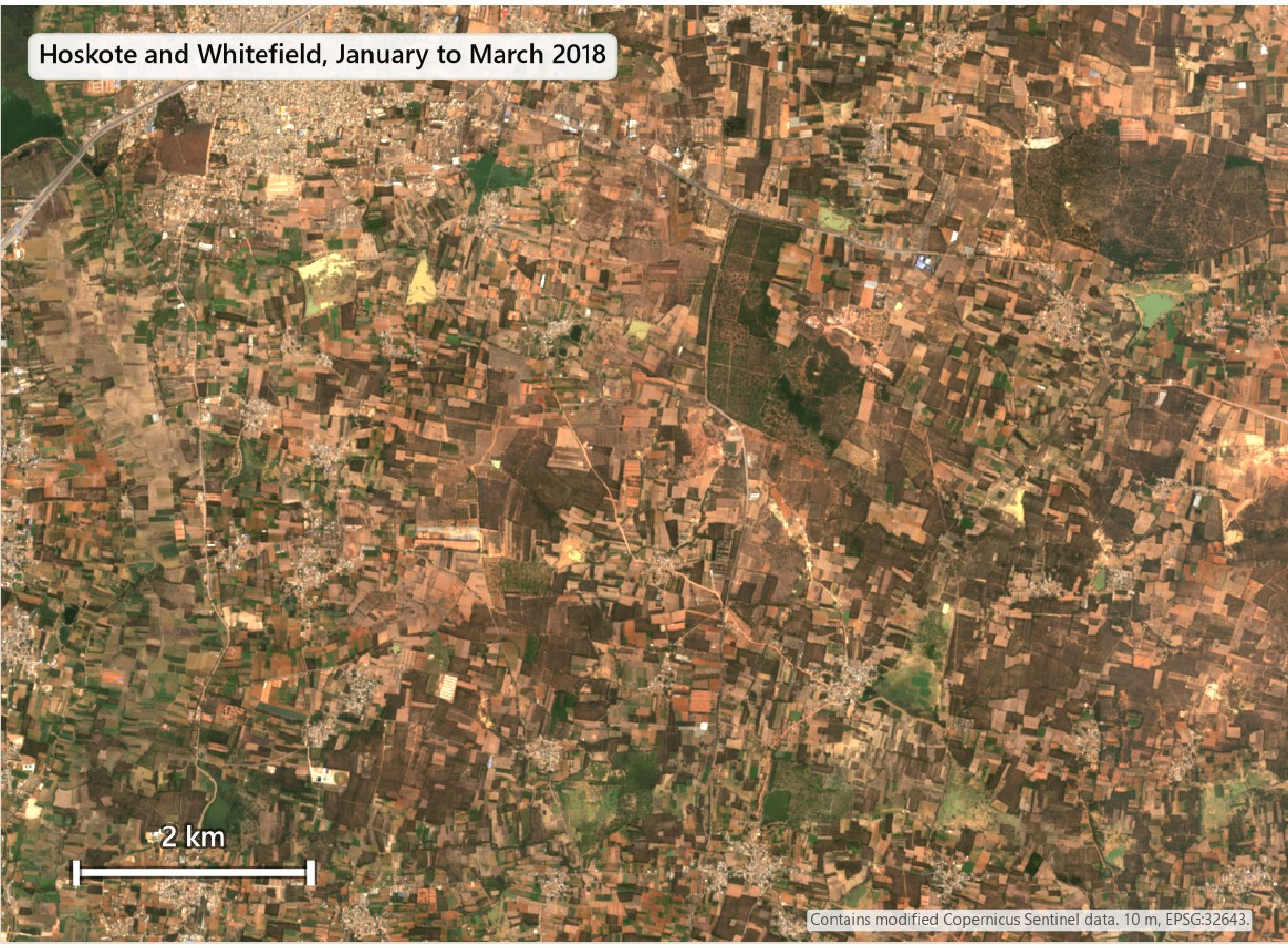
The colours differ between the two dates because they come from different scene mixes.
How accurate is it?
I checked the maps three ways.
First check: 300 random points
I drew 300 random points, six groups of 50, from the first version of the map, hid the map's answer and labelled each point by eye on Esri World Imagery, with an older Esri image for 2018. For 2026 the first map showed about 1,730 km² of built-up land. My labels support 850 km² (plus or minus 155 km²). The map found nearly every built point but called about half of its built pixels something else on the ground. Most of those were vacant or cleared plots, or trees and yards inside built blocks.
Second version, fresh sample
I built a stricter classifier with more land-cover classes and trained on pure pixels. Then I drew 150 new points, none used for training, and labelled them blind. The 2026 map agrees with my labels in 68% of the pixels it calls built (75% if cleared land counts as built). Its mapped area (about 1,070 km² in the design area) is still about 1.5 times what the labels support (721 km², plus or minus 112 km²). New built-up land is worse: the map shows 2.3 times the area my labels support (about 440 km² against 188 km²). The figures in the introduction come from these labels.
Third check: a re-look at mixed squares
Many 10 m squares turned out to be mixed, a roof next to a tree next to a plot. I re-labelled 60 of the points blind, giving a main class and, when the square was mixed, a second class. 25 of the 60 squares were mixed. My labels were fairly stable: on the 28 points where the classifier and my first label agreed, the second look gave the same main class 71% to 86% of the time, and on the 24 points where they disagreed it gave 88%. Of those 24 points, where the classifier said built and I had said not built, only one was built as the main class on the second look, but 42% had built as the main or the second class. So the classifier was mostly reading a building next to the square.
I tried one more thing, a third version that reports built-up share per 100 m cell and adds slope and an open-ground class. The pixel-level result was no better: it recovered only 5 of the 39 open or rock points. I did not validate the density version at the 100 m scale, so I do not quote numbers from it.
A longer view, and the Landsat cross-check
I also tried Landsat at 30 m for 2015 to 2025. Landsat reaches further back, but the 2015 composite is brighter than the later ones over land that did not change. With the same cut-off for both years, the net change from 2015 to 2025 runs from a loss of 88 km² to a gain of 95 km² depending on which cut-off I pick. With a separate calibrated cut-off for each year it is a gain of about 560 km². A result that moves that much with the cut-off is not a measurement, so I cannot give a number for that decade and include Landsat only as a warning.
Methodology
Study area, grid and data
The study area is Bengaluru Urban, Bengaluru Rural and Ramanagara districts (13 taluks). Boundaries come from geoBoundaries, which is built from the Local Government Directory: districts from the 2021 release and taluks from 2018. They add up to 7,904 km², against the official 8,005 km². Everything is projected to EPSG:32643 (UTM zone 43N) and held on one 10 m grid of about 13,900 by 9,400 pixels.
| Data | Used for |
|---|---|
| Sentinel-2 L2A, January to March 2018, 2022 and 2026 (Earth Search) | The maps |
| ESRI 10 m annual land cover 2017 to 2023 and ESA WorldCover 2020 and 2021 | Training labels and the earlier land cover of the new land |
| Copernicus GLO-30 elevation | Slope and the relief on the maps |
| OpenStreetMap motorways, trunk and primary roads | Distance to roads |
| Esri World Imagery and Esri Wayback | Labelling the validation points |
| Landsat Collection 2 Level-2 (Planetary Computer) | The 2015 to 2025 cross-check |
Image composites
For each year I took the clear Sentinel-2 scenes from 1 January to 31 March, kept only the pixels the scene classification layer labels as vegetation, bare ground, water, dark area or unclassified (so clouds, cloud shadow, cirrus, snow and saturated pixels are out), and took the per-pixel median of six bands (blue, green, red, near-infrared and two short-wave infrared). The 2026 composite comes from the newer Collection 1 archive. The 2018 and 2022 composites come from the original archive, because Collection 1 has too few clear scenes in those years. I checked every older scene for the brightness offset described above and corrected only the scenes that showed it. After that, the median brightness of land that did not change (cropland, grass and built-up land in both reference maps) agreed between 2018, 2021 and 2022 to within 0.01 in the short-wave infrared band I checked. 2026 came out slightly darker (a median of 0.30 against 0.32 to 0.33), which is one reason each year gets its own threshold.
Training data
The classifier learns from the 2021 composite. A pixel is a training example only if ESRI and WorldCover agree on its class and all eight neighbours carry the same label. The classes are built-up land, bare ground, cropland, vegetation and water. Cropland and vegetation examples also have to lie more than 100 m from any land that either map calls built. I sampled up to 150,000 pixels per class, 60,000 for water and about 16,000 for bare ground, because few pixels qualify. For the second version I added the 294 points from my first labelling round (leaving out the unclear ones) as extra examples with 50 times the weight of an ordinary pixel, plus 31 more built examples from the 2018 composite for points I had marked as already built in 2018.
Classifier
The model is a gradient-boosted decision tree (scikit-learn's HistGradientBoostingClassifier: 200 iterations, depth 8, learning rate 0.1). Its inputs are ten values per pixel and nothing from neighbouring pixels: the six bands, NDVI, NDBI, MNDWI and overall brightness. Versions that added neighbourhood means and texture over-counted more in my out-of-fold test, so I dropped them. The first version was a simple built or not-built model trained only on pixels where the two reference maps agree. The third version added slope, an open-ground class and per-hectare built-up density. I explain in the accuracy section why I do not quote numbers from it.
From probability to a built-up map
- For 2026 the threshold on the built-up probability is 70. I chose it as the highest value that still found 85% or more of the real built-up points in an out-of-fold test, which means the threshold choice used my labels. For 2018 (75) and 2022 (58) I set the threshold so that land that is certainly not built gets the same false-positive rate as in 2026 (0.87%). Certainly not built means cropland, or trees and rangeland, that both reference maps agree on and that lies more than 300 m from any land they call built.
- A pixel stays built only if at least five of the nine pixels in its 3 by 3 neighbourhood are built, and only if its connected patch has at least four pixels (0.04 ha). This removes isolated mixed pixels.
- A pixel counts as built in a year only if it is also built at the next date, and once built it stays built, so the map has no demolition. The last date has no next date, so land first counted in 2026 rests on one observation. The result is a raster of the first year each pixel is built.
Statistics
- Distance rings are 5 km wide, measured from Vidhana Soudha (77.5906 E, 12.9795 N).
- Taluk figures use the 13 taluk polygons.
- For roads, I measured the distance from each 40 m cell of new built-up land to the nearest OpenStreetMap motorway, trunk or primary road. For named roads I summed the new land within 2 km of them.
- For the earlier land cover of the new land, I read ESRI's 2018 map, the start of the period, and WorldCover 2020 under each new built-up pixel. For farmland I used ESRI 2018 crops and WorldCover 2020 cropland as two baselines.
- All of these statistics describe the map, which over-counts. They show where and when, not how much.
Validation
I labelled every point blind: the files showed no map output, and the answer key was kept in a separate folder. For each point I looked at a 10 m square on the latest Esri World Imagery and picked one class: built (roofs, roads, paved ground), vacant or cleared, cropland, vegetation, water, or unclear. For built or cleared points I then looked at Esri Wayback imagery near 2018 and answered whether a building or paved surface was already there.
| Round | Map checked | Points | Design |
|---|---|---|---|
| 1 | First version | 300 | Six groups drawn from the map, 50 points each: not built far from built land, not built near built land, new in 2018 to 2022, new in 2022 to 2026, built by 2018, and a probability band near the threshold |
| 2 | Second version | 150 | Five groups drawn from the frozen map: built by 2018 (30), new 2018 to 2022 (40), new 2022 to 2026 (40), not built far from built land (15) and not built near it (25). Points were at least 500 m inside the region edge and 100 m from round 1 points, and their IDs were shuffled. The classifier had never seen them |
| 3 | Re-check | 60 | Points from rounds 1 and 2 shown again without my first label, with a main class and an optional second class |
For the estimates I used stratified estimators (Cochran), where the area of each group weights its share of points that were built. A 95% interval is 1.96 times the standard error. User's accuracy is the share of mapped built-up land that was built, and producer's accuracy is the share of real built-up land that the map found. Both use ratio estimators with the same group areas. A point counts as built when I labelled it built. Cleared plots are reported separately, and "new" means built now and not built in 2018. I dropped the points I labelled unclear (3 of the 150).
Landsat cross-check
For the 2015 to 2025 interval I built Landsat composites at 30 m for 2015, 2021 and 2025, masked cloud with the quality band, matched the 2015 composite to 2021 brightness by quantiles over land that did not change, and ran the same kind of classifier. The change depended so much on the cut-off that I report it only as a warning.
Reproducing it
Everything is in Python (rasterio, GeoPandas, scikit-learn, SciPy and pystac-client). The scripts are numbered in run order, each writes its outputs to a named table or raster, and a stage log records every number and every failure.
Workflow
- Download the district and taluk polygons and project everything to EPSG:32643 (UTM zone 43N, metres), so that 10 m pixels and kilometre distances are true.
- Build a median of clear January to March Sentinel-2 observations for 2018, 2022 and 2026. Mask clouds with the scene classification layer. Check for the brightness offset in the older archive.
- Take the pixels where ESRI and WorldCover agree on built, cropland, vegetation, water and bare. Keep only pure pixels.
- Train a classifier on band values and indices, and predict every pixel of each year.
- Set each year's cut-off so that land that is certainly not built gets the same false-positive rate in every year.
- A pixel is built in a year if it is also built at the next date, and once built it stays built.
- Count area by distance ring, taluk, road distance and the farmland baseline.
- Draw a stratified random sample, label it blind, and compute accuracy and area estimates with confidence intervals.
Counting the area of a mapped class is short in Python. This reads the first-year-built raster and prints the area built by each year in square kilometres:
import numpy as np
import rasterio

with rasterio.open("first_year_built_v2_10m.tif") as src:
    first = src.read(1)              # 0 = not built, 65535 = outside the region
    pixel_km2 = abs(src.res[0] * src.res[1]) / 1e6

inside = first != 65535
for year in (2018, 2022, 2026):
    built = inside & (first > 0) & (first <= year)
    print(year, round(built.sum() * pixel_km2, 1), "km2 mapped as built")
The error-adjusted area is a weighted sum. For each sampling group, take the share of its labelled points that really were built, multiply by the group's area, and add the groups up. The groups are the strata of the sample, and the confidence interval comes from the spread inside each group.
Common mistakes
- Trusting the mapped area. A map can look right and still carry twice the area, and only a sample of independent points tells you how much.
- Using the same cut-off every year. Composites from different years shift in brightness, and equalising the false-positive rate on certainly-not-built land removed most of that shift. It did not equalise detection: the map found 78% of certainly-built land in 2018 and 83% in 2026, so the mapped change is a little too high, which is one more reason to quote the labelled estimate.
- Using NDBI in the dry season, when it flags dry fields as built-up land.
- Calling cleared land built. A cleared plot is not a building, so keep it as its own class.
- Judging one 10 m square. In a dense neighbourhood a square can fall on a tree or a gap, so allow a second class or report the built-up share over a larger cell.
- Trusting scene metadata for the brightness offset. In the older archive the metadata said to subtract 0.1, but many scenes did not contain the matching +1,000 and came out too dark. Check the data, for example with lake pixels.
Key takeaways
- Built-up land around Bengaluru grew by about 190 km² between 2018 and 2026 (about 260 km² including cleared plots), about a third more than in 2018. The maps show about 445 km², so they over-count.
- Most of the growth is 10 to 30 km from the city centre, and a third of it is within 500 m of a major road.
- The growth is largest in absolute terms in Bengaluru South, Anekal and Bengaluru North, and fastest in percentage terms in Devanahalli, Yelahanka and Hoskote.
- What the new land was before depends on the baseline map. WorldCover has about a third of it as cropland, while ESRI already shows most of it as built.
- At 10 m, built-up edges are mixed with trees, plots and soil. A map of those edges needs a sample of independent points to turn it into an area.
Limitations
- The sample has only 39 points in the 6,560 km² that the map calls not built, and none of them was built. The plus-or-minus figures describe sampling alone and cannot rule out that the map misses some built-up land there, so the area estimates are more likely too low than too high.
- The accuracy numbers come from points I labelled myself, with imagery of varying dates. Another person could label some points differently, as my re-check showed.
- The area estimates come from 150 points for the second version and 300 for the first, so the intervals are wide, especially for change.
- Pixels first counted as built in the last interval rest on one observation, so the 2022 to 2026 growth is less certain than the earlier interval.
- The third version, with density and an open-ground class, was checked only against labels I had already used for training.
- The second version learned from my first 294 labels, and I chose its 2026 threshold using them, so only the fresh sample of 150 points is an independent check of it.
- The reference maps I trained on (ESRI and WorldCover) are themselves model products with their own errors, and the rule that built land stays built cannot show demolition.
- This study measures land cover. It says nothing about legal land use, ownership or approvals.
Data and tools
- Sentinel-2 Level-2A (ESA/Copernicus), January to March 2018, 2022 and 2026, via Earth Search. Contains modified Copernicus Sentinel data.
- ESRI 10 m annual land cover (2017 to 2023) and ESA WorldCover 2020 and 2021, for training labels and baselines.
- Copernicus GLO-30 DEM for slope.
- OpenStreetMap roads, via Overpass (ODbL, © OpenStreetMap contributors).
- geoBoundaries (built from the Local Government Directory, ODbL) for districts and taluks.
- Esri World Imagery and Esri Wayback imagery for labelling.
- Landsat Collection 2 Level-2 via the Microsoft Planetary Computer, for the cross-check.
- Python with rasterio, GeoPandas, scikit-learn, SciPy and Matplotlib.